Markov random fields

Bayesian networks are a class of models that can compactly represent many interesting probability distributions. However, we have seen in the previous chapter that some distributions may have independence assumptions that cannot be perfectly represented by the structure of a Bayesian network.

In such cases, unless we want to introduce false independencies among the variables of our model, we must fall back to a less compact representation (which can be viewed as a graph with additional, unnecessary edges). This leads to extra, unnecessary parameters in the model, and makes it more difficult to learn these parameters and to make predictions.

There exists, however, another technique for compactly representing and visualizing a probability distribution that is based on the language of undirected graphs. This class of models (known as Markov Random Fields or MRFs) can compactly represent independence assumptions that directed models cannot represent. We will explore the advantages and drawbacks of these methods in this chapter.

Markov Random Fields

⊕
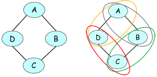
Undirected graphical representation of a joint probability of voting preferences over four individuals. The figure on the right illustrates the pairwise factors present in the model. As a motivating example, suppose that we are modeling voting preferences among persons $A,B,C,D$. Let’s say that $(A,B)$, $(B,C)$, $(C,D)$, and $(D,A)$ are friends, and friends tend to have similar voting preferences. These influences can be naturally represented by an undirected graph.

One way to define a probability over the joint voting decision of $A,B,C,D$ is to assign scores to each assignment to these variables and then define a probability as a normalized score. A score can be any function, but in our case, we will define it to be of the form

\[\tilde p(A,B,C,D) = \phi(A,B)\phi(B,C)\phi(C,D)\phi(D,A),\]

where $\phi(X,Y)$ is a factor that assigns more weight to consistent votes among friends $X,Y$, e.g.:

\[\begin{align*} \phi(X,Y) = \begin{cases} 10 & \text{if } X = Y = 1 \\ 5 & \text{if } X = Y = 0 \\ 1 & \text{otherwise}. \end{cases} \end{align*}\]

The factors in the unnormalized distribution are often referred to as factors. The final probability is then defined as

\[p(A,B,C,D) = \frac{1}{Z} \tilde p(A,B,C,D),\]

where $Z = \sum_{A,B,C,D} \tilde p(A,B,C,D)$ is a normalizing constant that ensures that the distribution sums to one.

When normalized, we can view $\phi(A,B)$ as an interaction that pushes $B$’s vote closer to that of $A$. The term $\phi(B,C)$ pushes $B$’s vote closer to $C$, and the most likely vote will require reconciling these conflicting influences.

Note that unlike in the directed case, we are not saying anything about how one variable is generated from another set of variables (as a conditional probability distribution would do). We simply indicate a level of coupling between dependent variables in the graph. In a sense, this requires less prior knowledge, as we no longer have to specify a full generative story of how the vote of $B$ is constructed from the vote of $A$ (which we would need to do if we had a $P(B\mid A)$ factor). Instead, we simply identify dependent variables and define the strength of their interactions; this in turn defines an energy landscape over the space of possible assignments and we convert this energy to a probability via the normalization constant.

Formal definition

A Markov Random Field (MRF) is a probability distribution $p$ over variables $x_1,...,x_n$ defined by an undirected graph $G$ in which nodes correspond to variables $x_i$. The probability $p$ has the form

\[p(x_1, \dotsc, x_n) = \frac{1}{Z} \prod_{c \in C} \phi_c(x_c),\]

where $C$ denotes the set of cliques (i.e. fully connected subgraphs) of $G$. The value

\[Z = \sum_{x_1, \dotsc, x_n} \prod_{c \in C} \phi_c(x_c)\]

is a normalizing constant that ensures that the distribution sums to one.

Thus, given a graph $G$, our probability distribution may contain factors whose scope is any clique in $G$, which can be a single node, an edge, a triangle, etc. Note that we do not need to specify a factor for each clique. In our above example, we defined a factor over each edge (which is a clique of two nodes). However, we chose not to specify any unary factors, i.e. cliques over single nodes.

Comparison to Bayesian networks

⊕
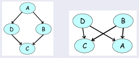
Examples of directed models for our four-variable voting example. None of them can accurately express our prior knowledge about the dependency structure among the variables. In our earlier voting example, we had a distribution over $A,B,C,D$ that satisfied $A \perp C \mid \{B,D\}$ and $B \perp D \mid \{A,C\}$ (because only friends directly influence a person’s vote). We can easily check by counter-example that these independencies cannot be perfectly represented by a Bayesian network. However, the MRF turns out to be a perfect map for this distribution.

More generally, MRFs have several advantages over directed models:

They can be applied to a wider range of problems in which there is no natural directionality associated with variable dependencies.
Undirected graphs can succinctly express certain dependencies that Bayesian nets cannot easily describe (although the converse is also true)

They also possess several important drawbacks:

Computing the normalization constant $Z$ requires summing over a potentially exponential number of assignments. We will see that in the general case, this will be NP-hard; thus many undirected models will be intractable and will require approximation techniques.
Undirected models may be difficult to interpret.
It is much easier to generate data from a Bayesian network, which is important in some applications.

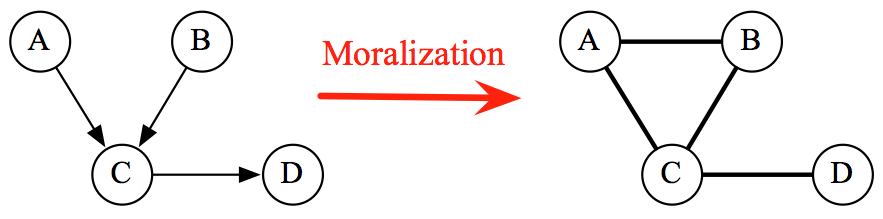
It is not hard to see that Bayesian networks are a special case of MRFs with a very specific type of clique factor (one that corresponds to a conditional probability distribution and implies a directed acyclic structure in the graph), and a normalizing constant of one. In particular, if we take a directed graph $G$ and add side edges to all parents of a given node (and removing their directionality), then the CPDs (seen as factors over a variable and its ancestors) factorize over the resulting undirected graph. The resulting process is called moralization.

A Bayesian network can always be converted into an undirected network with normalization constant one. The converse is also possible, but may be computationally intractable, and may produce a very large (e.g. fully connected) directed graph.

Thus, MRFs have more power than Bayesian networks, but are more difficult to deal with computationally. A general rule of thumb is to use Bayesian networks whenever possible, and only switch to MRFs if there is no natural way to model the problem with a directed graph (like in our voting example).

Independencies in Markov Random Fields

Recall that in the case of Bayesian networks, we defined a set of independencies $I(G)$ that were described by a directed graph $G$, and showed how these describe true independencies that must hold in a distribution $p$ that factorizes over the directed graph, i.e. $I(G) \subseteq I(p)$.

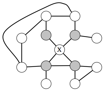
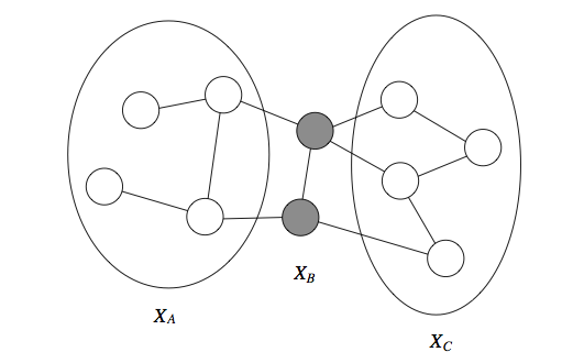
⊕ In an MRF, a node $$X$$ is independent from the rest of the graph given its neighbors (which are referred to at the Markov blanket of $$X$$.
In an MRF, a node $X$ is independent from the rest of the graph given its neighbors (which are referred to at the Markov blanket of $X$. What independencies can be then described by an undirected MRF? The answer here is very simple and intuitive: variables $x,y$ are dependent if they are connected by a path of unobserved variables. However, if $x$’s neighbors are all observed, then $x$ is independent of all the other variables, since they influence $x$ only via its neighbors.

In particular, if a set of observed variables forms a cut-set between two halves of the graph, then variables in one half are independent from ones in the other.

Formally, we define the Markov blanket $U$ of a variable $X$ as the minimal set of nodes such that $X$ is independent from the rest of the graph if $U$ is observed, i.e. $X \perp (\mathcal{X} - \{X\} - U) \mid U$. This notion holds for both directed and undirected models, but in the undirected case the Markov blanket turns out to simply equal a node’s neighborhood.

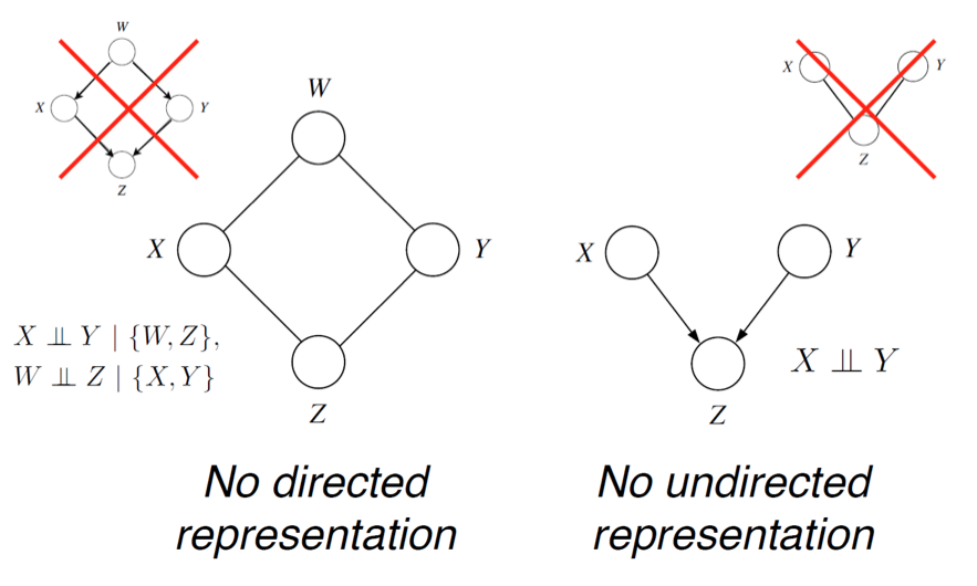
In the directed case, we found that $I(G) \subseteq I(p)$, but there were distributions $p$ whose independencies could not be described by $G$. In the undirected case, the same holds. For example, consider a probability described by a directed v-structure (i.e. the explaining away phenomenon). The undirected model cannot describe the independence assumption $X \perp Y$.

Examples of probability distributions that have a perfect directed graphical representation but no undirected representation, and vice-versa.

Conditional Random Fields (Skip for now)

An important In the interest of time we’ll skip discussion of CRFs in class, but they are an important example of how flexible PGMs can be. We may come back to them later in the course.special case of Markov Random Fields arises when they are applied to model a conditional probability distribution $p(y\mid x)$. In this case, $x \in \mathcal{X}$ and $y \in \mathcal{Y}$ are vector-valued variables; we are typically given $x$ and want to say something interesting for $y$. Typically, distributions of this sort will arise in a supervised learning setting, where $y$ will be a vector-valued label that we will be trying to predict. This setting is typically referred to as structured prediction.

Example

As a motivating example, consider the problem of recognizing a word from a sequence of character images $x_i \in [0, 1]^{d\times d}$ given to us in the form of pixel matrices. The output of our predictor will be a sequence of alphabet letters $y_i \in \{'a','b',...,'z'\}$.

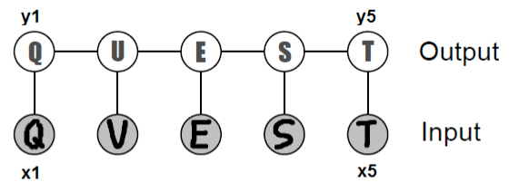
Chain-structured conditional random field for optical character recognition.

We could in principle train a classifier to separately predict each $y_i$ from its $x_i$. However, since the letters together form a word, the predictions across different $i$ ought to inform each other. In the above example, the second letter by itself could be either a ‘U’ or a ‘V’; however, since we can tell with high confidence that its neighbors are ‘Q’ and ‘E’, we can infer that ‘U’ is the most likely true label. CRFs are a tool that will enable us to perform this prediction jointly.

Formal definition

Formally, a CRF is a Markov network over variables $\mathcal X \cup \mathcal Y$ which specifies a conditional distribution

\[P(y\mid x) = \frac{1}{Z(x)} \prod_{c \in C} \phi_c(x_c,y_c)\]

with partition function

\[Z(x) = \sum_{y \in \mathcal{Y}} \prod_{c \in C} \phi_c(x_c,y_c).\]

Note that in this case, the partition constant now depends on $x$ (therefore, we say that it is a function), which is not surprising: $p(y\mid x)$ is a probability over $y$ that is parametrized by $x$, i.e. it encodes a different probability function for each $x$. In that sense, a conditional random field results in an instantiation of a new Markov Random Field for each input $x$.

Example (continued)

More formally, suppose $p(y\mid x)$ is a chain CRF with two types of factors: image factors $\phi(x_i, y_i)$ for $i = 1, ..., n$ — which assign higher values to $y_i$ that are consistent with an input $x_i$ — as well as pairwise factors $\phi(y_i, y_{i+1})$ for $i = 1, ..., n-1$. We may also think of the $\phi(x_i,y_i)$ as probabilities $p(y_i\mid x_i)$ given by, say, standard (unstructured) softmax regression; the $\phi(y_i, y_{i+1})$ can be seen as empirical frequencies of letter co-occurrences obtained from a large corpus of English text (e.g. Wikipedia).

Given a model of this form, we can jointly infer the structured label $y$ using MAP inference:

\[\arg\max_y \phi_1(y_1, x_1) \prod_{i=2}^n \phi(y_{i-1}, y_i) \phi(y_i, x_i).\]

CRF features

In most practical applications, we further assume that the factors $\phi_c(x_c,y_c)$ are of the form

\[\phi_c(x_c,y_c) = \exp(w_c^T f_c(x_c, y_c)),\]

where $f_c(x_c, y_c)$ can be an arbitrary set of features describing the compatibility between $x_c$ and $y_c$.

In our OCR example, we may introduce features $f(x_i, y_i)$ that encode the compatibility of the letter $y_i$ with the pixels $x_i$. For example, $f(x_i, y_i)$ may be the probability of letter $y_i$ produced by logistic regression (or a deep neural network) evaluated on pixels $x_i$. In addition, we introduce features $f(y_i, y_{i+1})$ between adjacent letters. These may be indicators of the form $f(y_i, y_{i+1}) = \Ind(y_i = \ell_1, y_{i+1} = \ell_2)$, where $\ell_1, \ell_2$ are two letters of the alphabet. The CRF would then learn weights $w$ that would assign more weight to more common probability of consecutive letters $(\ell_1, \ell_2)$, while at the same time making sure that the predicted $y_i$ are consistent with the input $x_i$; this process would let us determine $y_i$ in cases where $x_i$ is ambiguous, like in our above example.

The most important realization that need to be made about CRF features is that they can be arbitrarily complex. In fact, we may define an OCR model with factors $\phi_i(x,y_i) = \exp(w_i^T f(x, y_i))$, that depend on the entire input $x$. This will not affect computational performance at all, because at inference time, the $x$ will be always observed, and our decoding problem will involve maximizing

\[\phi_1(x, y_1) \prod_{i=2}^n \phi(y_{i-1}, y_i) \phi(x, y_i) = \phi_1'(y_1) \prod_{i=2}^n \phi(y_{i-1}, y_i) \phi'(y_i),\]

where $\phi'_i(y_i) = \phi_i(x,y_i)$. Using global features only changes the values of the factors, but not their scope, which possesses the same type of chain structure. We will see in the next section that this structure is all that is needed to ensure we can solve this optimization problem tractably.

This observation may be interpreted in a slightly more general form. If we were to model $p(x,y)$ using an MRF (viewed as a single model over $x, y$ with normalizing constant $Z = \sum_{x,y} \tp(x,y)$), then we need to fit two distributions to the data: $p(y\mid x)$ and $p(x)$. However, if all we are interested in is predicting $y$ given $x$, then modeling $p(x)$ is unnecessary. In fact, it may be disadvantageous to do so statistically (e.g. we may not have enough data to fit both $p(y\mid x)$ and $p(x)$; since the models have shared parameters, fitting one may result in the best parameters for the other) and it may not be a good idea computationally (we need to make simplifying assumptions in the distribution so that $p(x)$ can be handled tractably). CRFs forgo of this assumption, and often perform better on prediction tasks.

Factor Graphs

It is often useful to view MRFs in a way where factors and variables are explicit and separate in the representation. A factor graph is one such way to do this. A factor graph is a bipartite graph where one group is the variables in the distribution being modeled, and the other group is the factors defined on these variables. Edges go between factors and variables that those factors depend on.

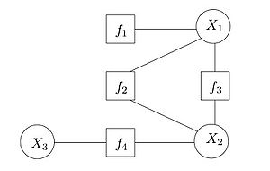
Example of a factor graph with three variables and four factors.

This view allows us to more readily see the factor dependencies between variables, and later we’ll see it allows us to compute some probability distributions more easily.

Index