Bayesian learning

The learning approaches we have discussed so far are based on the principle of maximum likelihood estimation. While being extremely general, there are limitations of this approach as illustrated in the two examples below.

Example 1

Let’s suppose we are interested in modeling the outcome of a biased coin, \(X = \{heads, tails\}\). We toss the coin 10 times, observing 6 heads. If \(\theta\) denotes the probability of observing heads, the maximum likelihood estimate (MLE) is given by, \(\theta_{MLE} = \frac{num\_heads}{num\_heads + num\_tails} = 0.6\)

Now, suppose we continue tossing the coin such that after a 100 total trials (including the 10 initial trials), we observe 60 heads. Again, we can compute the MLE as,

In both the above situations, the maximum likelihood estimate does not change as we observe more data. This seems counterintuitive - our confidence in predicting heads with probability 0.6 should be higher in the second setting where we have seen many more trials of the coin! The reason why MLE fails to distinguish the two settings is due to an implicit assumption it makes. MLE assumes that the only source of uncertainty is due to the variables, \(X\) and the quantification of this uncertainty is based on a fixed parameter \(\theta_{MLE}\).

Example 2

Consider a language model for sentences based on the bag-of-words assumption. In such a model, the probability of a sentence can be factored as the probability of the words appearing in the sentence.

For simplicity, assume that our language corpus consists of a single sentence, “Probabilistic graphical models are fun. They are also powerful.” We can estimate the probability of each of the individual words based on the counts. Our corpus contains 10 words with each word appearing once, and hence, each word in the corpus is assigned a probability of 0.1. Now, while testing the generalization of our model to the English language, we observe another sentence, “Probabilistic graphical models are hard.” The probability of the sentence under our model is \(0.1 \times 0.1 \times 0.1 \times 0.1 \times 0 = 0\). We did not observe one of the words (“hard”) during training which made our language model infer the sentence as impossible, even though it is a perfectly plausible sentence.

Out-of-vocabulary words are a common phenomena even for language models trained on large corpus. One of the simplest ways to handle these words is to assign a prior probability of observing an out-of-vocabulary word such that the model will assign a low, but non-zero probability to test sentences containing such words. This mechanism of incorporating prior knowledge is a practical application of Bayesian learning, which we present next.

Setup

In contrast to maximum likelihood learning, Bayesian learning explicitly models uncertainty over both the variables, \(X\) and the parameters, \(\theta\). In other words, the model parameters \(\theta\) are random variables as well.

A prior distribution over the parameters, \(p(\theta)\) encodes our initial beliefs. These beliefs are subjective. For example, we can choose the prior over \(\theta\) for a biased coin to be uniform between 0 and 1. If however we expect the coin to be fair, the prior distribution can be peaked around \(\theta = 0.5\). We will discuss commonly used priors later in this chapter.

Observing data \(D\) in the form of evidence allows us to update our beliefs using Bayes’ rule,

Hence, Bayesian learning provides a principled mechanism for incorporating prior knowledge into our model. This prior knowledge is useful in many situations such as when want to provide uncertainty estimates about the model parameters (Example 1) or when the data available for learning a model is limited (Example 2).

Conjugate Priors

When calculating posterior distribution using Bayes’ rule, as in the above, it should be pretty straightforward to calculate the numerator. But to calculate the denominator \(P(D)\), we are required to compute an integral. This might cause us trouble, since for an arbitrary distribution, computing the integral is likely to be intractable.

To tackle this issue, we use a conjugate prior. A parametric family \(\varphi\) is conjugate for the likelihood \(P(D \mid \theta)\) if:

This is convenient because if we know the normalizing constant of \(\varphi\), then we get the denominator in Bayes’ rule “for free”. Thus it essentially reduces the computation of the posterior from a tricky numerical integral to some simple algebra.

To see conjugate prior in action, let’s consider an example. Suppose we are given a sequence of \(N\) coin tosses, \(D = \{X_{1},\ldots,X_{N}\}\). We want to infer the probability of getting heads which we denote by \(\theta\). Now, we can model this as a sequence of Bernoulli trials with parameter \(\theta\). A natural conjugate prior in this case is the beta distribution with

where the normalization constant \(B(\cdot)\) is the beta function. Here \(\alpha = (\alpha_H,\alpha_T)\) are called the hyperparameters of the prior. The expected value of \(\theta\) is \(\frac{\alpha_H}{\alpha_H+\alpha_T}\). Here the sum of the hyperparameters \((\alpha_H+\alpha_T)\) can be interpreted as a measure of confidence in the expectations they lead to. Intuitively, we can think of \(\alpha_H\) as the number of heads we have observed before the current dataset.

⊕
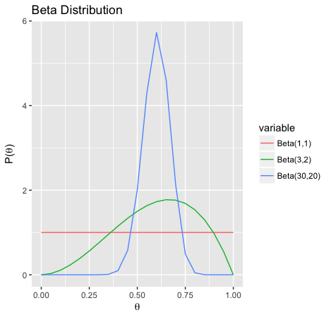
Here the exponents \((3,2)\) and \((30,20)\) can both be used to encode the belief that \(\theta\) is \(0.6.\) But the second set of exponents imply a stronger belief as they are based on a larger sample.

Out of \(N\) coin tosses, if the number of heads and the number of tails are \(N_H\) and \(N_T\) respectively, then it can be shown that the posterior is:

which is another Beta distribution with parameters \((N_H + \alpha_H, N_T + \alpha_T)\). We can use this posterior distribution as the prior for more samples with the hyperparameters simply adding each extra piece of information as it comes from additional coin tosses.

Categorical Generalization

We can now extend the binary model to its categorical generalization. Instead of being limited to binary outcomes, we can now consider the categorical dataset of a \(K\)-sided dice rolled \(N\) times. Let \(\mathcal{D} = \{ X_1 = k_1, \ldots, X_N = K_N \}\), where \(X_j \in \{ 1, \ldots, K \}\) for the \(j\)th outcome. The parameterization of the model is \(\theta = (P(X_j = 1), \ldots, P(X_j = K))\), which denotes the probability of each outcome, and where \(\sum_{k = 1}^K P(X_j = k) = 1\).

The likelihood of observing our dataset given a specific parameterization is

In the same manner as with the binary model, the conjugate prior for this categorical model is the Dirichlet distribution, which has hyperparameters \(\mathbf{\alpha} = (\alpha_1, \ldots, \alpha_K)\), indicating the number of observations of each outcome. Letting \(\alpha\) be the “virtual” counts of the \(K\) outcomes before we observe the dataset, our prior is

where \(B(\cdot)\) is still a normalization factor.

Because we use a Dirichlet prior, the posterior is also a Dirichlet distribution, and is formulated as follows:

We can see that this is equivalent to a Dirichlet distribution with updated counts \(\alpha'\). Specifically,

where the updated count \(\alpha'\) is given by