Map inference

This section will explore the problem of MAP inference in graphical models. MAP inference in a graphical model \(p\) corresponds to the following optimization problem:

The framework we have introduced for marginal inference now lets us easily perform MAP inference as well. The key observation is that the sum and max operators both distribute over products. Thus, replacing sums in marginal inference with maxes, we are able to solve the MAP inference problem.

For example, we may compute the partition function of a chain MRF as follows:

To compute the maximum value \(\tp^*\) of \(\tp(x_1, \dotsc, x_n)\), we simply replace sums with maxes, i.e.

Since both problems decompose in the same way, we may reuse all of the machinery developed for marginal inference and apply it directly to MAP inference. Note that this also applies to factor trees.

There is a small caveat in that we often want not just maximum value of a distribution, i.e. \(\max_x p(x)\), but also its most probable assignment, i.e. \(\arg\max_x p(x)\). This problem can be easily solved by keeping back-pointers during the optimization procedure. For instance, in the above example, we would keep a backpointer to the best assignment to \(x_1\) given each assignment to \(x_2\), a pointer to the best assignment to \(x_2\) given each assignment to \(x_3,\) and so on.

The challenges of MAP inference

Since we are maximizing the variable of \(p(x)\) you will usually see the log form used, since maximizing the logarithm of a function will yield the same value as maximizing the function itself.

where \(\theta_c(\bfx_c) = \log\phi_c(\bfx_c)\). Since \(Z\) is a constant this lets us easily ignore that term

In a way, MAP inference is easier than marginal inference. One reason for this is that the intractable partition constant \(\log Z\) does not depend on \(x\) and can be ignored:

Marginal inference can also be seen as computing and summing all assignments to the model, one of which is the MAP assignment. If we replace summation with maximization, we can also find the assignment with the highest probability; however, there exist more efficient methods than this sort of enumeration-based approach. The notes on Belief propagation (which is optional reading) show briefly how to solve this problem exactly within the same message passing framework as marginal inference. Here we look at more efficient specialized methods.

Nonetheless, the MAP problem is easier than general inference, in the sense that there are some models in which MAP inference can be solved in polynomial time, while general inference is NP-hard.

Examples

Many interesting examples of MAP inference are instances of structured prediction, which involves doing inference in a conditional random field (CRF) model \(p(y \mid x)\):

⊕
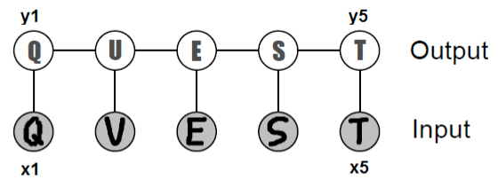
Chain-structured conditional random field for optical character recognition. See the optional CRF section of Markov random fields for more detail on this. One example of this handwriting recognition, in which we are given images \(x_i \in [0, 1]^{d\times d}\) of characters in the form of pixel matrices; MAP inference in this setting amounts to jointly recognizing the most likely word \((y_i)_{i=1}^n\) encoded by the images.

Another example of MAP inference is image segmentation; here, we are interested in locating an entity in an image and label all its pixels. Our input \(\bfx \in [0, 1]^{d\times d}\) is a matrix of image pixels, and our task is to predict the label \(y \in \{0, 1\}^{d\times d}\), indicating whether each pixel encodes the object we want to recover. Intuitively, neighboring pixels should have similar values in \(\bfy\), i.e. pixels associated with the horse should form one continuous blob (rather than white noise). ⊕
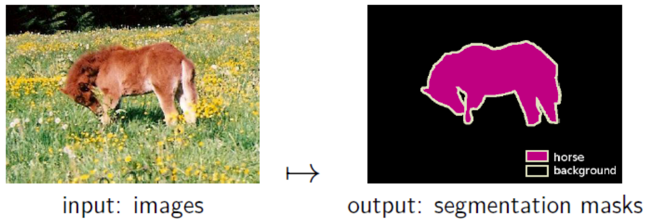
An illustration of the image segmentation problem.

This prior knowledge can be naturally modeled in the language of graphical models via a Potts model. As in our first example, we can introduce potentials \(\phi(y_i,x)\) that encode the likelihood that any given pixel is from our subject. We then augment them with pairwise potentials \(\phi(y_i, y_j)\) for neighboring \(y_i, y_j\), which will encourage adjacent \(y\)’s to have the same value with higher probability.

Solution Methods

Formulating this problem does not provide an efficient solution directly.

Graph Cuts

A graph cut of an undirected graph \(G = (V, \mathcal{E})\) is a partition of \(V\) into 2 disjoint sets \(V_s\) and \(V_t\). When each edge \((v_1, v_2) \in \mathcal{E}\) is associated with a nonnegative cost \(cost(v_1, v_2)\), the cost of a graph cut is the sum of the costs of the edges that cross between the two partitions:

The min-cut problem is to find the partition \(V_s, V_t\) that minimizes the cost of the graph cut. The fastest algorithms for computing min-cuts in a graph take \(O(\lvert \mathcal{E} \rvert \lvert V \rvert \log \lvert V \rvert)\) or \(O(\lvert V \rvert^3)\) time, and we refer readers to algorithms textbooks for details on their implementation.

MAP inference can be reduced to the min-cut problem in certain restricted cases of MRFs with binary variables.

Linear programming-based approaches

An approximate approach to computing the MAP values is to use Integer Linear Programming or Lagrangian optimization by introducing:

• indicator variables for each variable in the PGM
• indicator variables for each edge (or clqique) in the PGM
• constraints on consistent values in cliques, probabilities summing to 1, etc. Such a system is then solved using one of many linear optimization methods. Expensive for large systems but solution methods becoming more powerfull all the time.

Local search

A more heuristic-type solution consists in starting with an arbitrary assignment and perform “moves” on the joint assignment that locally increase the probability. This technique has no guarantees; however, we can often use prior knowledge to come up with highly effective moves. Therefore, in practice, local search may perform extremely well. A popular example is Broyden–Fletcher–Goldfarb–Shanno (BFGS) algorithm which is a quasi-Newton method for performing local search. This method approximates the second derivative of the underlying system and searches for a point where it is zero (ie. the minimum) to stop searching. This is the default for the find_MAP function in PyMC we will use later.

Branch and bound

Alternatively, one may perform exhaustive search over the space of assignments, while pruning branches that can be provably shown not to contain a MAP assignment. The LP relaxation or its dual can be used to obtain upper bounds useful for pruning trees.

Simulated annealing

A third approach is to use sampling methods (e.g. Metropolis-Hastings) to sample from \(p_t(x) \propto \exp(\frac{1}{t} \sum_{c \in C} \theta_c (x_c ))\). The parameter \(t\) is called the temperature. When \(t \to \infty\), \(p_t\) is close to the uniform distribution, which is easy to sample from. As \(t \to 0\), \(p_t\) places more weight on \(\arg\max_\bfx \sum_{c \in C} \theta_c (x_c )\), the quantity we want to recover. However, since this distribution is highly peaked, it is also very difficult to sample from.

The idea of simulated annealing is to run a sampling algorithm starting with a high \(t\), and gradually decrease it, as the algorithm is being run. If the “cooling rate” is sufficiently slow, we are guaranteed to eventually find the mode of our distribution. In practice, however, choosing the rate requires a lot of tuning. This makes simulated annealing somewhat difficult to use in practice.