Junction tree algorithm
We have seen how the variable elimination (VE) algorithm can answer marginal queries of the form \(P(Y \mid E = e)\) for both directed and undirected networks.
However, this algorithm has an important shortcoming: if we want to ask the model for another query, e.g. \(P(Y_2 \mid E_2 = e_2)\), we need to restart the algorithm from scratch. This is very wasteful and computationally burdensome.
Fortunately, it turns out that this problem is also easily avoidable. When computing marginals, VE produces many intermediate factors \(\tau\) as a side-product of the main computation; these factors turn out to be the same as the ones that we need to answer other marginal queries. By caching them after a first run of VE, we can easily answer new marginal queries at essentially no additional cost.
The end result of this chapter will be a new technique called the Junction Tree (JT) algorithmIf you are familiar with dynamic programming (DP), you can think of VE vs. the JT algorithm as two flavors of same technique: top-down DP v.s. bottom-up table filling. Just like in computing the \(n\)-th Fibonacci number \(F_n\), top-down DP (i.e. VE) computes just that number, but bottom-up (i.e. JT) will create a filled table of all \(F_i\) for \(i \leq n\). Moreover, the two-pass nature of JT is a result of the underlying DP on bi-directional (junction) trees, while Fibonacci numbers’ relation is a uni-directional tree.; this algorithm will first execute two runs of the VE algorithm to initialize a particular data structure holding a set of pre-computed factors. Once the structure is initialized, it can answer marginal queries in \(O(1)\) time.
We will introduce two variants of this algorithm: belief propagation (BP), and the full junction tree method. BP applies to tree-structured graphs, while the junction-tree method is applicable to general networks.
Belief propagation
Variable elimination as message passing
First, consider what happens if we run the VE algorithm on a tree in order to compute a marginal \(p(x_i)\). We can easily find an optimal ordering for this problem by rooting the tree at \(x_i\) and iterating through the nodes in post-orderA postorder traversal of a rooted tree is one that starts from the leaves and goes up the tree such that a node is always visited after all of its children. The root is visited last..
This ordering is optimal because the largest clique formed during VE will have size 2. At each step, we will eliminate \(x_j\); this will involve computing the factor \(\tau_{jk}(x_k) = \sum_{x_j} \phi(x_k, x_j) \tau_j(x_j)\), where \(x_k\) is the parent of \(x_j\) in the tree. At a later step, \(x_k\) will be eliminated, and \(\tau_{jk}(x_k)\) will be passed up the tree to the parent \(x_l\) of \(x_k\) in order to be multiplied by the factor \(\phi(x_l, x_k)\) before being marginalized out. The factor \(\tau_j(x_j)\) can be thought of as a message that \(x_j\) sends to \(x_k\) that summarizes all of the information from the subtree rooted at \(x_j\). We can visualize this transfer of information using arrows on a tree.
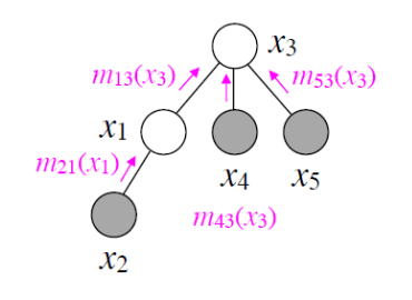
Message passing order when using VE to compute \(p(x_3)\) on a small tree.
At the end of VE, \(x_i\) receives messages from all of its immediate children, marginalizes them out, and we obtain the final marginal.
Now suppose that after computing \(p(x_i)\), we want to compute \(p(x_k)\) as well. We would again run VE with \(x_k\) as the root, waiting until \(x_k\) receives all messages from its children. The key insight: the messages \(x_k\) received from \(x_j\) now will be the same as those received when \(x_i\) was the rootAnother reason why this is true is because there is only a single path connecting two nodes in the tree.. Thus, if we store the intermediary messages of the VE algorithm, we can quickly recompute other marginals as well.
A message-passing algorithm
The key question here: how exactly do we compute all the messages we need? Notice for example, that the messages to \(x_k\) from the side of \(x_i\) will need to be recomputed.
The answer is very simple: a node \(x_i\) sends a message to a neighbor \(x_j\) whenever it has received messages from all nodes besides \(x_j\). It’s a fun exercise to the reader to show that in a tree, there will always be a node with a message to send, unless all the messages have been sent out. This will happen after precisely \(2 \vert E \vert\) steps, since each edge can receive messages only twice: once from \(x_i \to x_j\), and once more in the opposite direction.
Finally, this algorithm will be correct because our messages are defined as the intermediate factors in the VE algorithm.
We are now ready to formally define the belief propagation algorithm. This algorithm has two variants, each used for a different task:
- sum-product message passing: used for marginal inference, i.e. computing \(p(x_i)\)
- max-product message passing: used for MAP (maximum a posteriori) inference, i.e. computing \(\max_{x_1, \dotsc, x_n} p(x_1, \dotsc, x_n)\)
Sum-product message passing
The sum-product message passing algorithm is defined as follows: while there is a node \(x_i\) ready to transmit to \(x_j\), send the message
\[m_{i\to j}(x_j) = \sum_{x_i} \phi(x_i) \phi(x_i,x_j) \prod_{\ell \in N(i) \setminus j} m_{\ell \to i}(x_i).\]The notation \(N(i) \setminus j\) refers to the set of nodes that are neighbors of \(i\), excluding \(j\). Again, observe that this message is precisely the factor \(\tau\) that \(x_i\) would transmit to \(x_j\) during a round of variable elimination with the goal of computing \(p(x_j)\).
Because of this observation, after we have computed all messages, we may answer any marginal query over \(x_i\) in constant time using the equation
\[p(x_i) \propto \phi(x_i) \prod_{\ell \in N(i)} m_{\ell \to i}(x_i).\]Sum-product message passing for factor trees
Sum-product message passing can also be applied to factor trees with a slight modification. Recall that a factor graph is a bipartite graph with edges going between variables and factors, with an edge signifying a factor depends on a variable.
On factor graphs, we have two types of messages: variable-to-factor messages \(\nu\) and factor-to-variable messages \(\mu\). Both messages require taking a product, but only the factor-to-variable messages \(\mu\) require a sum.
\[\nu_{var(i)\to fac(s)}(x_i) = \prod_{t\in\mathcal N(i)\setminus s}\mu_{fac(t)\to var(i)}(x_i) \\ \mu_{fac(s)\to var(i)}(x_i) = \sum_{x_{\mathcal N(s)\setminus i}}f_s(x_{\mathcal N(s)})\prod_{j\in\mathcal N(s)\setminus i}\nu_{var(j)\to fac(s)}(x_j)\]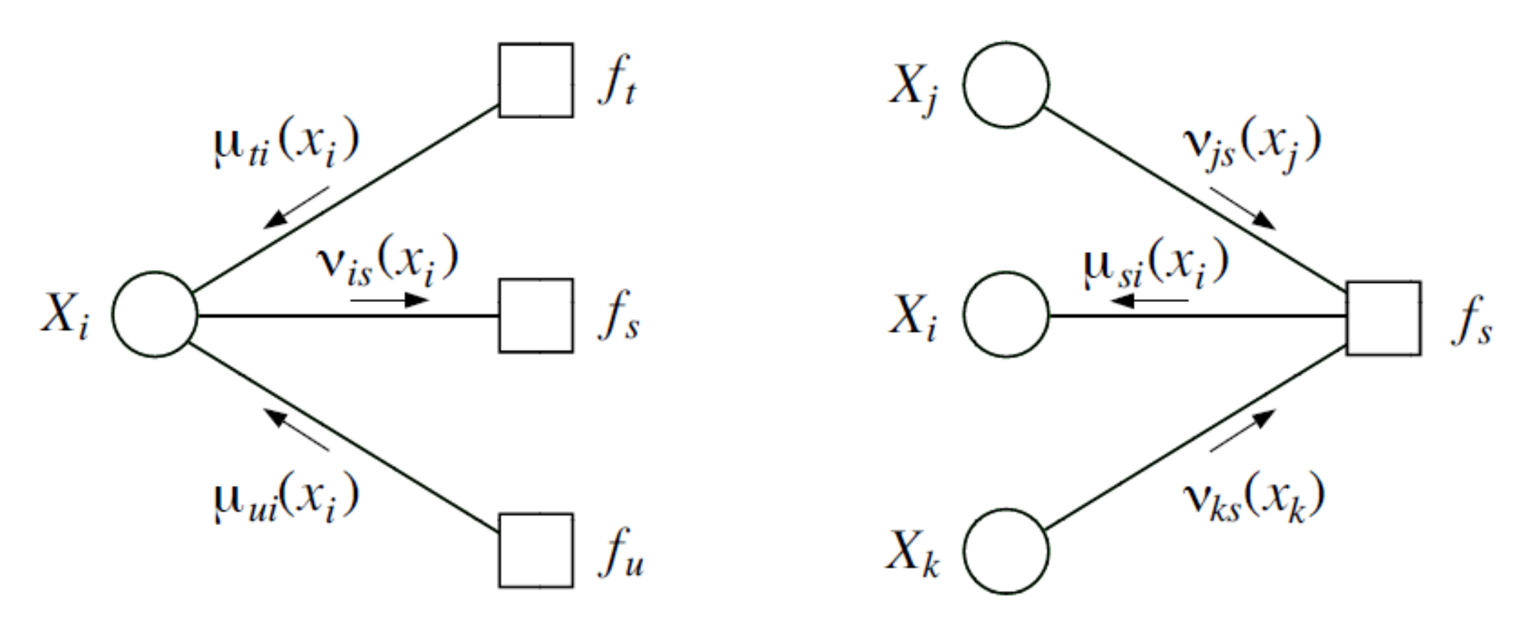
The algorithm proceeds in the same way as with undirected graphs: as long as there is a factor (or variable) ready to transmit to a variable (or factor), send the appropriate factor-to-variable (or variable-to-factor) message as defined above.
Max-product message passing
The second variant of the belief propagation algorithm, called max-product message passing, is used to perform MAP inference
\[\max_{x_1, \dotsc, x_n} p(x_1, \dotsc, x_n).\]The framework we have introduced for marginal inference now lets us easily perform MAP inference as well. The key observation is that the sum and max operators both distribute over products. Thus, replacing sums in marginal inference with maxes, we are able to solve the MAP inference problem.
For example, we may compute the partition function of a chain MRF as follows:
\[\begin{align*} Z &= \sum_{x_1} \cdots \sum_{x_n} \phi(x_1) \prod_{i=2}^n \phi(x_i, x_{i-1}) \\ &= \sum_{x_n} \sum_{x_{n-1}} \phi(x_n, x_{n-1}) \sum_{x_{n-2}} \phi(x_{n-1}, x_{n-2}) \cdots \sum_{x_1} \phi(x_2 , x_1) \phi(x_1) . \end{align*}\]To compute the maximum value \(\tp^*\) of \(\tp(x_1, \dotsc, x_n)\), we simply replace sums with maxes, i.e.
\[\begin{align*} \tp^* &= \max_{x_1} \cdots \max_{x_n} \phi(x_1) \prod_{i=2}^n \phi(x_i, x_{i-1}) \\ &= \max_{x_n} \max_{x_{n-1}} \phi(x_n, x_{n-1}) \max_{x_{n-2}} \phi(x_{n-1}, x_{n-2}) \cdots \max_{x_1} \phi(x_2 , x_1) \phi(x_1) . \end{align*}\]Since both problems decompose in the same way, we may reuse all of the machinery developed for marginal inference and apply it directly to MAP inference. Note that this also applies to factor trees.
There is a small caveat in that we often want not just maximum value of a distribution, i.e. \(\max_x p(x)\), but also its most probable assignment, i.e. \(\arg\max_x p(x)\). This problem can be easily solved by keeping back-pointers during the optimization procedure. For instance, in the above example, we would keep a backpointer to the best assignment to \(x_1\) given each assignment to \(x_2\), a pointer to the best assignment to \(x_2\) given each assignment to \(x_3,\) and so on.
Junction tree algorithm
So far, our discussion assumed that the graph is a tree. What if that is not the case? Inference in that case will not be tractable; however, we may try to massage the graph to its most tree-like form, and then run message passing on this graph.
At a high-level the junction tree algorithm partitions the graph into clusters of variables; internally, the variables within a cluster could be highly coupled; however, interactions among clusters will have a tree structure, i.e. a cluster will be only directly influenced by its neighbors in the tree. This leads to tractable global solutions if the local (cluster-level) problems can be solved exactly.
An illustrative example
Before we define the full algorithm, we start with an example, like we did for the variable elimination algorithm.
Suppose that we are performing marginal inference on an MRF of the form
\[p(x_1, \dotsc, x_n) = \frac{1}{Z} \prod_{c \in C} \phi_c(x_c),\]Crucially, we assume that the cliques \(c\) some path structure, meaning that we can find an ordering \(x_c^{(1)}, \dotsc, x_c^{(n)}\) with the property that if \(x_i \in x_c^{(j)}\) and \(x_i \in x_c^{(k)}\) for some variable \(x_i\) then \(x_i \in x_c^{(\ell)}\) for all \(x_c^{(\ell)}\) on the path between \(x_c^{(j)}\) and \(x_c^{(k)}\). We refer to this assumption as the running intersection property (RIP).
Suppose that we are interested in computing the marginal probability \(p(x_1)\) in the above example. Given our assumptions, we may again use a form of variable elimination to “push in” certain variables deeper into the product of cluster potentials:
\[\phi(x_1) \sum_{x_2} \phi(x_1,x_2) \sum_{x_3} \phi(x_1,x_2,x_3) \sum_{x_5} \phi(x_2,x_3,x_5) \sum_{x_6} \phi(x_2,x_5,x_6).\]We first sum over \(x_6\), which creates a factor \(\tau(x_2, x_3, x_5) = \phi(x_2,x_3,x_5) \sum_{x_6} \phi(x_2,x_5,x_6)\). Then, \(x_5\) gets eliminated, and so on. At each step, each cluster marginalizes out the variables that are not in the scope of its neighbor. This marginalization can also be interpreted as computing a message over the variables it shares with the neighbor.
The running intersection property is what enables us to push sums in all the way to the last factor. We may eliminate \(x_6\) because we know that only the last cluster will carry this variable: since it is not present in the neighboring cluster, it cannot be anywhere else in the graph without violating the RIP.
Junction trees
The core idea of the junction tree algorithm is to turn a graph into a tree of clusters that are amenable to the variable elimination algorithm like the above MRF. Then we simply perform message-passing on this tree.
Suppose we have an undirected graphical model \(G\) (if the model is directed, we consider its moralized graph). A junction tree \(T=(C, E_T)\) over \(G = (\Xc, E_G)\) is a tree whose nodes \(c \in C\) are associated with subsets \(x_c \subseteq \Xc\) of the graph vertices (i.e. sets of variables); the junction tree must satisfy the following properties:
- Family preservation: For each factor \(\phi\), there is a cluster \(c\) such that \(\text{Scope}[\phi] \subseteq x_c\).
- Running intersection: For every pair of clusters \(c^{(i)}, c^{(j)}\), every cluster on the path between \(c^{(i)}, c^{(j)}\) contains \(x_c^{(i)} \cap x_c^{(j)}\).
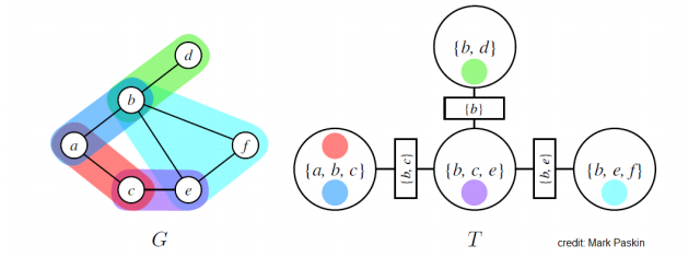
Here is an example of an MRF with graph \(G\) and junction tree \(T\). MRF potentials are denoted using different colors; circles indicates nodes of the junction trees; rectangular nodes represent sepsets (short for “separation sets”), which are sets of variables shared by neighboring clusters.
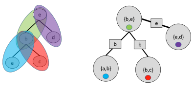
A junction tree defined over a tree graph. Clusters correspond to edges.
Example of an invalid junction tree that does not satisfy the running intersection property.
Note that we may always find a trivial junction tree with one node containing all the variables in the original graph. However, such trees are useless because they will not result in efficient marginalization algorithms.
Optimal trees are one that make the clusters as small and modular as possible; unfortunately, it is again NP-hard to find the optimal tree. We will see below some practical ways in which we can find good junction trees.
A special case when we can find the optimal junction tree is when \(G\) itself is a tree. In that case, we may define a cluster for each edge in the tree. It is not hard to check that the result satisfies the above definition.
The junction tree algorithm
We now define the junction tree algorithm and explain why it works. At a high-level, this algorithm implements a form of message passing on the junction tree, which will be equivalent to variable elimination for the same reasons that BP was equivalent to VE.
More precisely, let us define the potential \(\psi_c(x_c)\) of each cluster \(c\) as the product of all the factors \(\phi\) in \(G\) that have been assigned to \(c\). By the family preservation property, this is well-defined, and we may assume that our distribution is in the form
\[p(x_1, \dotsc, x_n) = \frac{1}{Z} \prod_{c \in C} \psi_c(x_c).\]Then, at each step of the algorithm, we choose a pair of adjacent clusters \(c^{(i)}, c^{(j)}\) in \(T\) and compute a message whose scope is the sepset \(S_{ij}\) between the two clusters:
\[m_{i\to j}(S_{ij}) = \sum_{x_c \backslash S_{ij}} \psi_c(x_c) \prod_{\ell \in N(i) \backslash j} m_{\ell \to i}(S_{\ell i}).\]We choose \(c^{(i)}, c^{(j)}\) only if \(c^{(i)}\) has received messages from all of its neighbors except \(c^{(j)}\). Just as in belief propagation, this procedure will terminate in exactly \(2 \lvert E_T \rvert\) steps. After it terminates, we will define the belief of each cluster based on all the messages that it receives
\[\beta_c(x_c) = \psi_c(x_c) \prod_{\ell \in N(i)} m_{\ell \to i}(S_{\ell i}).\]These updates are often referred to as Shafer-Shenoy. After all the messages have been passed, beliefs will be proportional to the marginal probabilities over their scopes, i.e. \(\beta_c(x_c) \propto p(x_c)\). We may answer queries of the form \(\tp(x)\) for \(x \in x_c\) by marginalizing out the variable in its beliefReaders familiar with combinatorial optimization will recognize this as a special case of dynamic programming on a tree decomposition of a graph with bounded treewidth.
\[\tp(x) = \sum_{x_c \backslash x} \beta_c(x_c).\]To get the actual (normalized) probability, we divide by the partition function \(Z\) which is computed by summing all the beliefs in a cluster, \(Z = \sum_{x_c} \beta_c(x_c)\).
Note that this algorithm makes it obvious why we want small clusters: the running time will be exponential in the size of the largest cluster (if only because we may need to marginalize out variables from the cluster, which often must be done using brute force). This is why a junction tree of a single node containing all the variables is not useful: it amounts to performing full brute-force marginalization.
Variable elimination over a junction tree
Why does this method work? First, let us convince ourselves that running variable elimination with a certain ordering is equivalent to performing message passing on the junction tree; then, we will see that the junction tree algorithm is just a way of precomputing these messages and using them to answer queries.
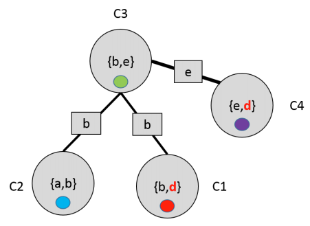
Suppose we are performing variable elimination to compute \(\tp(x')\) for some variable \(x'\), where \(\tp = \prod_{c \in C} \psi_c\). Let \(c^{(i)}\) be a cluster containing \(x'\); we will perform VE with the ordering given by the structure of the tree rooted at \(c^{(i)}\). In the example below, say that we choose to eliminate the \(b\) variable, and we set \((a,b,c)\) as the root cluster.
First, we pick a set of variables \(x_{-k}\) in a leaf \(c^{(j)}\) of \(T\) that does not appear in the sepset \(S_{kj}\) between \(c^{(j)}\) and its parent \(c^{(k)}\) (if there is no such variable, we may multiply \(\psi(x_c^{(j)})\) and \(\psi(x_c^{(k)})\) into a new factor with a scope not larger than that of the initial factors). In our example, we may pick the variable \(f\) in the factor \((b,e,f)\).
Then we marginalize out \(x_{-k}\) to obtain a factor \(m_{j \to k}(S_{ij})\). We multiply \(m_{j \to k}(S_{ij})\) with \(\psi(x_c^{(k)})\) to obtain a new factor \(\tau(x_c^{(k)})\). Doing so, we have effectively eliminated the factor \(\psi(x_c^{(j)})\) and the unique variables it contained. In the running example, we may sum out \(f\) and the resulting factor over \((b, e)\) may be folded into \((b,c,e)\).
Note that the messages computed in this case are exactly the same as those of JT. In particular, when \(c^{(k)}\) is ready to send its message, it will have been multiplied by \(m_{\ell \to k}(S_{ij})\) from all neighbors except its parent, which is exactly how JT sends its message.
Repeating this procedure eventually produces a single factor \(\beta(x_c^{(i)})\), which is our final belief. Since VE implements the messages of the JT algorithm, \(\beta(x_c^{(i)})\) will correspond to the JT belief. Assuming we have convinced ourselves in the previous section that VE works, we know that this belief will be valid.
Formally, we may prove correctness of the JT algorithm through an induction argument on the number of factors \(\psi\); we will leave this as an exercise to the reader. The key property that makes this argument possible is the RIP; it assures us that it’s safe to eliminate a variable from a leaf cluster that is not found in that cluster’s sepset; by the RIP, it cannot occur anywhere except that one cluster.
The important thing to note is that if we now set \(c^{(k)}\) to be the root of the tree (e.g. if we set \((b,c,e)\) to be the root), the message it will receive from \(c^{(j)}\) (or from \((b,e,f)\) in our example) will not change. Hence, the caching approach we used for the belief propagation algorithm extends immediately to junction trees; the algorithm we formally defined above implements this caching.
Finding a good junction tree
The last topic that we need to address is the question of constructing good junction trees.
- By hand: Typically, our models will have a very regular structure, for which there will be an obvious solution. For example, very often our model is a grid, in which case clusters will be associated with pairs of adjacent rows (or columns) in the grid.
- Using variable elimination: One can show that running the VE elimination algorithm implicitly generates a junction tree over the variables. Thus it is possible to use the heuristics we previously discussed to define this ordering.
Loopy belief propagation
As we have seen, the junction tree algorithm has a running time that is potentially exponential in the size of the largest cluster (since we need to marginalize all the cluster’s variables). For many graphs, it will be difficult to find a good junction tree, applying the algorithm will not be possible. In other cases, we may not need the exact solution that the junction tree algorithm provides; we may be satisfied with a quick approximate solution instead.
Loopy belief propagation (LBP) is another technique for performing inference on complex (non-tree structure) graphs. Unlike the junction tree algorithm, which attempted to efficiently find the exact solution, LBP will form our first example of an approximate inference algorithm.
Definition for pairwise models
Suppose that we are given an MRF with pairwise potentialsArbitrary potentials can be handled using an algorithm called LBP on factor graphs. We will include this material at some point in the future.. The main idea of LBP is to disregard loops in the graph and perform message passing anyway. In other words, given an ordering on the edges, at each time \(t\) we iterate over a pair of adjacent variables \(x_i, x_j\) in that order and simply perform the update
\[m^{t+1}_{i\to j}(x_j) = \sum_{x_i} \phi(x_i) \phi(x_i,x_j) \prod_{\ell \in N(i) \setminus j} m^{t}_{\ell \to i}(x_i).\]We keep performing these updates for a fixed number of steps or until convergence (the messages don’t change). Messages are typically initialized uniformly.
Properties
This heuristic approach often works surprisingly well in practice.
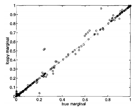
Marginals obtained via LBP compared to true marginals obtained from the JT algorithm on an intensive care monitoring task. Results are close to the diagonal, hence very similar.
In general, however, it may not converge and its analysis is still an area of active research. We know for example that it provably converges on trees and on graphs with at most one cycle. If the method does converge, its beliefs may not necessarily equal the true marginals, although very often in practice they will be close.
We will return to this algorithm later in the course and try to explain it as a special case of variational inference algorithms.
| Index | Previous | Next |